local illumination models

The first attempts resulted in what we're calling today a ``local illumination model''. These are widely used in today's PC 3D graphic adapter technology (OpenGL and DirectX are famous software libraries providing 3D graphic primitive operations, mainly polygon-based, with local illumination models).

Local illumination models mainly introduce two simplifications:

1. The objects will be rendered isolated from their environment; in the moment of rendering no other objects are taken into account. This results in having no inter-reflections etc. at all!
2. Only reflections are taken into account (transparency could be imitated with tricky algorithm, but it remains a fake).

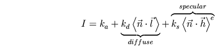
A famous algorithm for local illumination models is Phong's formula describing diffuse and specular reflections:

$$I = k_a+\underbrace{k_d\left<\vec{n}\cdot\vec{l} \right>}_{... ...}+\overbrace{k_s\left<\vec{n}\cdot\vec{h}\right>^e}^{specular}$$ (1)

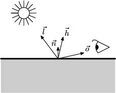
Figure 2: Vectors in a local illumination model

Equation 1 separates the intensity of the percepted light in three components:

ambiental component

represents the background illumination, i.e. light being diffused by other objects. You could see it as a very simple approximation for a radiosity solution (therefore you shouldn't use ambiental components when using radiosity!). Thus it is represented by the additive ambiental intensity $k_a$.

diffuse component

represents the reflected light diffused by the rough microstructure of the surface. Following the observation that the diffuse component reaches its maximum when the lightsource shones at the surfaces vertically and its minimum when the rays are in parallel with the surface its intensity will be approximated by the scalar product of the vector pointing to the lightsource $\vec{l}$ and the norm vector of the surface $\vec{n}$ (see fig. 2. The factor $k_d$ rules the strength of the diffuse component as a material property.

specular component

represents the light reflected by even parts of the microstructure. It will be maximal when the observer position lies in the path ruled by the reflection law. Therefore we could use the scalar product of the vector describing the reflected light path (could be calculated by "mirroring" $\vec{l}$ at $\vec{n}$) with the vector $\vec{o}$; for computational efficency the scalar product of the norm vector $\vec{n}$ and a helping vector $\vec{h}$

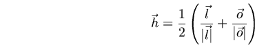$$\vec{h} = \frac{1}{2}\left(\frac{\vec{l}}{\vert\vec{l}\vert} +\frac{\vec{o}}{\vert\vec{o}\vert}\right)$$ (2)

will be used instead.

Notice that the separation of reflections into diffuse and specular components has no physical background!

Equation 1 also shows the importance of the norm vector $\vec{n}\;$ in the lightning calculation; indeed $\vec{n}\;$ is used to simulate an uneven surface via bump mapping.

To figure out the disadvantages of local illumination models have a look at the pictures 3,4,5; they've been rendered from the same scene, but with pure local illumination (pic. 3), a global illumination model (whitted-raytracing) taking global specular interreflections into account (pic. 4) and a global illumination model (radiosity plus two-way raytracing) which supports some combinations of diffuse and specular interreflections (pic. 5).

Figure 3: pure local illumination

Figure 4: Whitted-Raytracing

Figure 5: raytracing+radiosity

Notice that the local illumination model doesn't support shadows! If shadows are required for computer games etc. an additional rendering step has to be performed (usually following the observation that a shadowed surface isn't visible from the position of the lightsource drawing the shadow - which lead to a shadow-zbuffer technique which goes beyound the scope of this document).